Referential and Reviewed International Scientific-Analytical Journal of Ivane Javakhishvili Tbilisi State University, Faculty of Economics and Business


Estimating Capital Stock and Return on Capital for Georgia
Acknowledgement: This work was supported by the Shota Rustaveli National Science Foundation (SRNSF) [N FR17_122, The Puzzle of Economic Development without Rural Urban Migration in Georgia]
Abstract
In this paper, we estimate capital stock for Georgia using the Perpetual Inventory Model (PIM). Due to data constraints, different techniques are used to estimate the model’s parameters. The model is based on public and private annual investment data from 1996-2017. Georgia’s Statistics Office doesn’t publish official capital stock data, a key variable in estimating aggregate production function which is essential for economic growth models, productivity analysis, and many other macroeconomic applications. Thus, our work will contribute to different macroeconomic models on forecasting and policy analysis for Georgia. The second part of the paper presents the calculation of return on capital using the newly constructed capital stock series and uses the rate of return on capital series to try to understand what affected business investment demand in Georgia on a national level from 1999-2017.
Keywords: Capital Stock Estimation, Perpetual Inventory Model, Return on Capital, Business Investment.
JEL Codes: G32, H54, R53
Introduction
The Perpetual Inventory Model (PIM) was first introduced by Raymond W. Goldsmith in 1951, when he formulated the basic approach for how to measure national wealth in the United States. The basic idea of PIM is that it starts with an initial asset figure and adds investment in assets to fixed assets year by year (using gross fixed capital formation data), while controlling for annual depreciation. All data is adjusted for inflation using an investment deflator (or capital expenditure price index).
Researchers acknowledge that it is extremely difficult to get an accurate measure of capital stock for a country, since even a single firm owner may find it difficult to know what the assets are currently worth. The most difficult part of capital stock estimation is estimating the depreciation rate of different types of assets, since depreciation is not directly observable or measurable. Thus, different papers rely on a number of considerably different assumptions to overcome this problem. One needs to be careful about making international comparisons using capital stock data. Even the OECD database of capital stock is collected from member countries’ national statistical offices, and one should thoroughly research the underlying assumptions in order to make country comparisons.
Because of the complexity of the task, researchers have only made a few attempts to construct big capital stock databases. In 1993, Nehru and Dhareshwar constructed capital stock data for 93 countries from 1960-1990. Later, in 2000, De la Fuente and Domenech constructed capital stock data for OECD countries from 1950-1997. Most recently, in 2012, Berlemann and Wesselhöft used a holistic approach to estimate capital stock data for 103 countries from 1979-2010. All of these papers used the perpetual inventory model, but unfortunately none of them included Georgia on the list of selected countries. Thus, our paper contributes to the literature by constructing real capital stock estimates for Georgia using an internationally accepted methodology.
The first attempt at estimating capital stock for Georgia was done in 2017 by the National Bank of Georgia (NBG), based on the same perpetual inventory method using quarterly data from 1996-2016. NBG used an annual depreciation rate of 5%; however, no justification was provided, and they didn't control for external shocks (like the 2008 war with Russia, which changed the path of capital stock accumulation) in their model. Most importantly, NBG didn't provide a breakdown of capital stock by private and public capital stocks. Unlike NBG, we also adjust Gross Fixed Capital formation to account only for productive investments (we exclude investment in dwellings).
The paper is organized as follows. In section 2, we describe the PIM method in detail. Section 3 describes the available data, followed by estimating the model’s parameters in section 4. In section 5, we estimate return on capital using the capital stock series from section 4, and in the last section of the paper we use the rate of return on capital series to estimate a business investment function to understand what affected business investment demand in Georgia.
1. Methodology
Capital is one of the key inputs in the production function and it is provided by assets with useful life over a number of years. Thus, measuring the available capital for the production process requires information about the investments made over a period of time and previous investments aggregated using some methodology in which estimates of depreciation play the key role. In this section, we describe the methodology of capital stock calculation and in the following section we estimate the parameters of this model.
In order to calculate real capital stock in the country, we use the Perpetual Inventory Method, a commonly established methodology for measuring capital stock widely in practice, particularly by the European System of Accounts (ESA, 2010) and the OECD (OECD, 2001) [1], assuming that in the beginning of each period capital stock (available for the production process in that year) equals the sum of the gross capital stock at the beginning of the previous period less depreciation and investment from the previous period.
Where![]() is the value of net capital stock available at the beginning of period t+1
is the value of net capital stock available at the beginning of period t+1![]() is a (constant) geometric rate of depreciation, as there is little evidence that can be used to discriminate among different depreciation profiles used to estimate net capital stock. However, the assumption of a constant depreciation rate can still be maintained if there is evidence that the asset composition of capital stock does not change much over time. In this case, one can construct the constant
is a (constant) geometric rate of depreciation, as there is little evidence that can be used to discriminate among different depreciation profiles used to estimate net capital stock. However, the assumption of a constant depreciation rate can still be maintained if there is evidence that the asset composition of capital stock does not change much over time. In this case, one can construct the constant ![]() as a weighted average of depreciation rates of different types of assets contributing to the capital stock.
as a weighted average of depreciation rates of different types of assets contributing to the capital stock. ![]() is Gross Capital formation (capital formation and investment are synonyms and we will be using them interchangeably in this paper) in period t. Thus, to calculate capital stock we need the depreciation rate, time series investment data, and initial capital stock. For any country time series, investment data will be limited to some number of years and we need some method to estimate what the country’s initial capital stock was. We will also need to gauge the depreciation rate of capital.
is Gross Capital formation (capital formation and investment are synonyms and we will be using them interchangeably in this paper) in period t. Thus, to calculate capital stock we need the depreciation rate, time series investment data, and initial capital stock. For any country time series, investment data will be limited to some number of years and we need some method to estimate what the country’s initial capital stock was. We will also need to gauge the depreciation rate of capital.
The first, steady state approach of estimating initial capital stock was introduced by Harberger (1978). This approach relies on the assumption that the economy is in a steady state. Using this assumption, from formula (1) the capital growth rate from t to t+1 can be expressed as follows:
With we denote growth of capital stock from the t to t+1 period. From formula (2) the value of capital stock in period t can be written as:
![]() 3)
3)
We use formula (3) to estimate capital stock in the initial period. The problem of this approach is that initial capital stock will depend on the single year growth rate and investment in that initial year, so even a small investment shock in that year will cause significant overestimation. To avoid the bias caused by the cyclical variation of investments, we apply the Berlemann & Wesselhöft (2014) approach to eliminate the effect of the current business cycle on the initial capital stock measure. According to Berlemann & Wesselhöft (2014) initial capital stock can be expressed as:
![]() (4)
(4)
Where ![]() is the initial capital stock
is the initial capital stock![]() , is the long-run growth rate of capital stock and
, is the long-run growth rate of capital stock and ![]() is the estimated investment from the following log-level regression:
is the estimated investment from the following log-level regression:
To calculate ![]() we need to plug in t=0, thus
we need to plug in t=0, thus ![]() and the growth rate is equal to
and the growth rate is equal to ![]() coefficient of the same regression. In order to calculate Ko the only remaining parameter
coefficient of the same regression. In order to calculate Ko the only remaining parameter ![]() – the depreciation rate. We partly rely on the literature to calculate the most relevant depreciation rate for capital stock in Georgia (see Estimation section).
– the depreciation rate. We partly rely on the literature to calculate the most relevant depreciation rate for capital stock in Georgia (see Estimation section).
2. Data
Public and private annual investment data for 1996-2017 comes from the Ministry of Finance of Georgia. Private investment is Gross Capital Formation, which includes Gross Fixed Capital Formation and Changes in Inventories. Starting from 2010, GeoStat also provided the breakdown of Gross Fixed Capital Formation into the following asset groups: Dwellings, Buildings other than dwellings, Other structures, Land improvements, Transport equipment, ICT equipment, Other machinery and equipment, Animal resources yielding repeat products, Tree, crop and plant resources yielding repeat products, Computer software, and Other intellectual property products. We group them into five categories.
Gross Fixed Capital Formation by Type of Assets
Figure 1
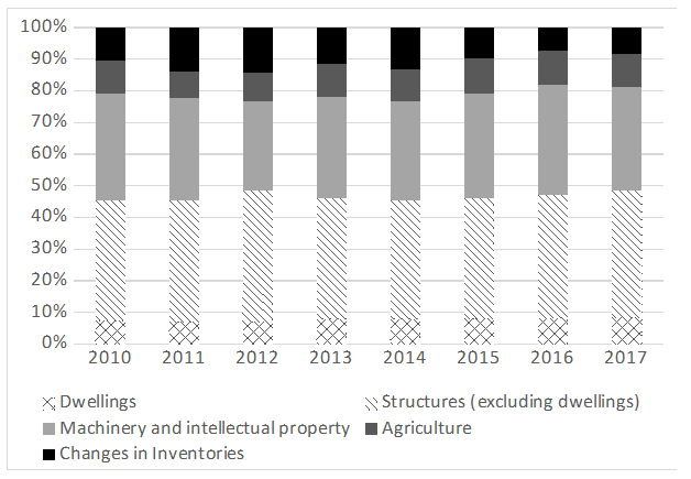
Source: GeoStat
Figure 1 shows that the share of Dwellings doesn’t vary much and stays within the 7-8% range of Gross Fixed Capital formation. Thus, we assume that it had the same pattern in previous years as well. We use the same shares to construct private investment series for the previous years (1996-2009) and then fully exclude the Dwelling category from private investment (but we still refer to this series as Private Investment in this paper from now on). This breakdown of Gross Fixed Capital Formation by types of asset is essential to estimate the depreciation rate for our model. To do so, we analyze the depreciation profiles of different types of assets.
In order to estimate the depreciation rate precisely, we need to know the prices of used assets and the expected life of assets, but data on used asset prices are not available in Georgia, thus we rely on literature and estimates from the Revenue Service of Georgia to calculate the weighted average depreciation rate. It is worth noting that depreciation estimates from tax codes were originally used in North America, but later they started to make use of used-asset prices and generated more precise estimates using econometric techniques.
For structures (excluding dwellings) we use a depreciation rate of 5%, and for the machinery category we use 20%, as these rates are used by the Revenue Service of Georgia (RS) for accounting purposes[2] and we also find similar estimates in the literature. There is a vast literature documenting that assets in the machinery category, unlike structures, exhibit substantial reduction in asset value, which is the reason for the substantially higher depreciation rate. Baldwin (2005) analyzed the 1961-1996 capital stock data of Canada and the estimated depreciation rate for machinery and equipment is at around 20% and around 10% for structures. Hulten (1981) reports a 13.3% depreciation rate for equipment and 3.7% for structures based on empirical evidence for the US economy in 1977. Levy (1995) explored time-varying capital stock depreciation rates for the post-war U.S. economy in all three main categories: consumer durable goods, producer durable goods, and business structures. He found that there has been no significant change in the depreciation rate of nonresidential business structures since the mid-1950s and it fluctuates around 5%, while the depreciation rate for producer durable goods increased over time and reached around 15.7% in 1991, as compared to 11.7% in 1948. Statistics Canada’s publication “Depreciation Rates for Productivity Accounts” (2007) is based on a number of applied studies measuring the depreciation rate and capital formation. They use three different methods (survival model, two-step technique, simultaneous technique) to estimate the depreciation rate for 240 separate assets from 1996-2001. They find that the average depreciation rate for machinery and equipment using different methods varies between 19.1-20%[3], and the average depreciation rate for buildings varies between 8.7-11.5%.
The Food and Agriculture Organization (FAO) adopted the perpetual inventory method to calculate agricultural capital stock, but due to the lack of information (usually used asset prices are not available) FAO uses δ=8% for OECD countries and δ between 4% and 8% for developing countries. Thus, we use a 5% depreciation rate for agricultural capital stock in Georgia.
Considering the shares of these different types of assets in private investment (Figure 1), we calculate that the weighted average annual depreciation rate is about 11%.
Assets and Depreciation Rate by Type of Assets
Figure 2
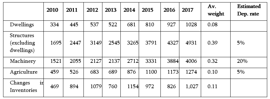
We don’t know the composition of inventories and exclude it from calculating the depreciation rate, which is equivalent to assuming that other categories are proportional to their size share in inventories. While a breakdown of public investment is not available, we use the same depreciation rate for public investments as well.
3. Estimating Capital Stock Series
To estimate the equation (5) separately for public and private investments, we convert the annual investment data to constant 2010 prices using the investment deflator. The investment deflator for 2003-2017 was estimated by the National Bank of Georgia[4] and we apply the 2-year moving average to construct the investment deflator for the previous years, which is a better fit compared to a different number of lags and linear approximation.
The drop in private investment during 2008-2009 was caused by the military intervention of Russia in Georgia in August 2008. Thus, we modify regression (5) by adding a war dummy as an explanatory variable (the war dummy has a value of 1 in 2008 and 2009 and 0 otherwise) to control for the war effect
Estimation results are shown in the table below:
Least Square Regression Results
Figure 3
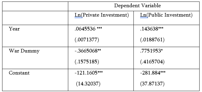
Note: ***, **, and * denote statistical significance levels at 1%, 5%, and 10%, respectively. Std. Err. reported in ( ).
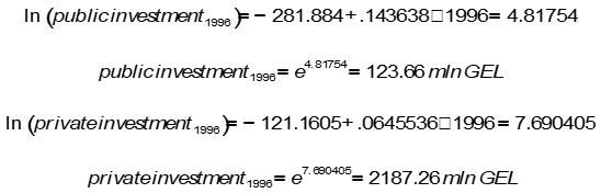
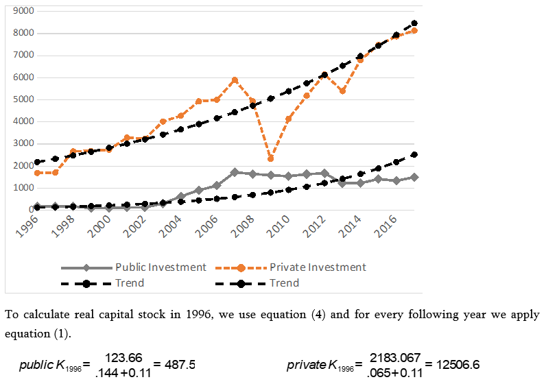
According to the regression results, the long-run growth rate of private investments is around 6.4% and is 14.4% for public investment. Using the regression results, we can also estimate initial, 1996, private and public investments ![]() that we need to calculate the initial capital stock according to formula (4):
that we need to calculate the initial capital stock according to formula (4):
Public and Private Investment (without dwellings) in 2010 prices (mln GEL) and trends based on Least Square Regression Results
Figure 4
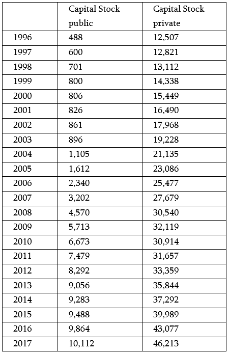
Public and Private capital stock, 1996-2017 (mln GEL, 2010 price
Figure 5
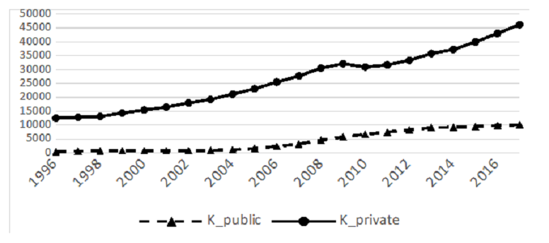
Both, private and public capital stock data are nonstationary. We used an Augmented Dickey–Fuller test to test capital stock time series data for random walk. As expected, we fail to reject the null hypothesis of a random walk with possible drift.
The capital series estimated according to the methodology described above can be used as an input in a variety of macroeconomic models. Below, we illustrate one of the practical applications, using the capital stock series to derive the rate of return on capital in Georgia between 1996 and 2017 and then using the estimated variable to explain the desired business investment at the country level from 1999-2017.
4. Estimating Return on Capital
In this section, we estimate the return on capital (ROC). The ROC is commonly defined as the ratio of profits generated by capital (or capital income) during a particular time period to the stock of capital. For the purposes of this exercise, profits on capital are estimated using the Net Operating Surplus 1996-2017 annual data from GeoStat, Generation of Income Account[5]. Thus, the return on capital is defined as Net Operating Surplus divided by total capital stock (public + private, excluding housing), both measured in constant 2010 prices[6]:

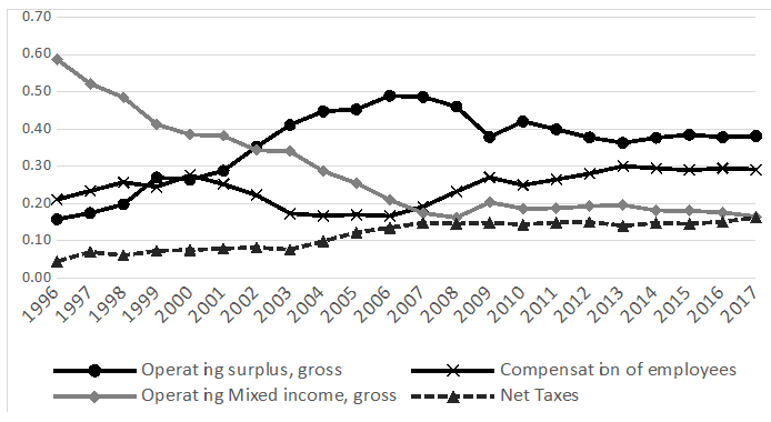
As a first step, we provide information on the evolution of capital, labor and other income shares in total GDP of Georgia between 1996 and 2017 (Figure 6). According to the income approach, the country’s Gross Domestic Product at market prices can be calculated as the sum of compensation of employees, net taxes on production and imports, gross operating surplus, and gross operating mixed income.
Generation of income account, shares of GDP at market prices.
Figure 6
 (7)
(7)
Source: GeoStat
According to GeoStat, compensation of employees is defined as remuneration, in cash and/or in kind, payable to employees for work completed during the accounting period. This component has increased over time and stabilized at 30% of GDP level over the last few years. Compensation of employees consists of wages and salaries (which include income taxes) and employers’ social contributions[7] even if they are actually withheld by the employer and paid directly to tax authorities, social security schemes and pension schemes. Besides wages that are regularly and directly paid to employees, wages and salaries also contain wages in kind, bonuses, overtime pay, tips, and commissions.
Net taxes is calculated as a difference between taxes on production and imports and subsidies on production. For this component, there were three phases: stable before 2004 at around 8% of GDP, growth during 2004-2007 reaching 15% of GDP, and stable again at around the same level.
Gross operating surplus is calculated as the balancing item in the generation of income account. Theoretically, that is the portion of income earned by the capital factor that is part of the value added which remains with producers after deducting expenditures related to the compensation of employees and taxes on production. Gross operating surplus less consumption of fixed capital[8] gives us Net Operating Surplus (NOS).
Gross Operating mixed income is a surplus generated as a result of production activity of unincorporated enterprises owned by households (informal sector). It reflects both remuneration of work done by the owner of the enterprise and entrepreneurial income as well. Generation of income account data is measured in current mln GEL; we use the investment deflator to convert NOS into constant 2010 prices.
Figure 7 presents the results of ROC calculations for Georgia as defined in equation (7).
Return on Capital
Figure 7
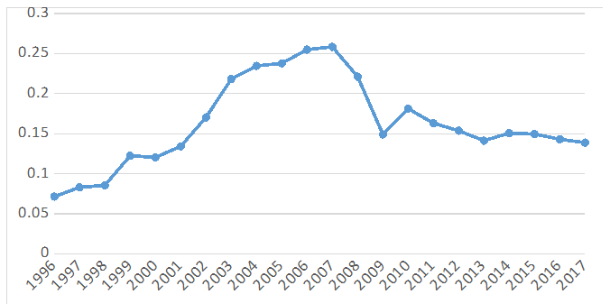
Source: GeoStat and own calculations
As one can see, return on capital exhibits a large range of variation, between 7-26%. The ROC increased from about 6% in 1996 to almost 26% in 2008, however it dropped significantly over the next two years as a result of the 2008 war with Russia and stabilized at around 14% over the last several years. According to the literature, rates of returns to capital tend to be quite stable in developed countries. For example, some studies report a rather narrow range of variation between 8-11% over 2013-2015 in Germany, Finland, the Czech Republic, and Greece (Canales, 2017). Empirical literature suggests that the results are quite different for developing economies and specifically for transition economies. For example, Chou, Izyumov and Vahaly (2018), estimated the rates of return on capital in the total of 109 countries, including highly developed countries (HDC), less developed countries (LDC) and transition (post-communist) economies (TEC) between 1994-2014. This study found that the return on capital was indeed much higher in LDC than in HDC, as the theory would suggest (ranging from 21% to 14.9% in LDC and from 12.7% to 10.1% in HDC). However, in the post-communist transition economies the rates of return on capital were initially close to those of HDC (11.7% in 1994), despite the fact that these countries were considered “capital poor” in the 1990s, and, in theory, should have had a higher ROC. One of the reasons for the low rate of return on capital was a much lower capital efficiency than in less-developed countries, such as Argentina, Brazil, Mexico, etc. (represented by the lower Y/K ratio). The rates of return on capital in TECs increased between 2001-2007 from about 12 to 15 percent and subsequently fell back to 11.4% by 2014.
The pattern for Georgia which is presented in our paper is generally consistent with the average findings for the transitional economies, albeit exhibiting much high degree of variation over time. In Georgia, as shown in Figure 7, the substantial increase in the return on capital described for other transition economies in 2001-2007 started from 13.4% and peaked at 25.6% in 2007.
5. Estimating Business Investment Function
In this section, we use rate of return on capital series to try to understand what affected business investment demand in Georgia on a country level between 1999 and 2017. Our empirical model of aggregate private business investment is based on the established theoretical frameworks for explaining private investment decisions, namely the q-theory of investment (Hall and Jorgenson (1967), Hayashi (1982)). The q-theory framework remains one of the most widespread, due to its strong micro-theoretical underpinnings. The baseline textbook model states that a profit-maximizing firm will invest until the point where its marginal revenue product of capital (captured by the rate of return on capital variable we estimated in the previous section) is equal to the user cost of capital, which is defined as the real interest rate multiplied by the relative price of capital goods (Burda and Wyplosz (2017), Romer (2018)). Thus, “marginal q”, which in theory captures all the relevant information about the firm’s investment decisions, is the difference between the rate of return on capital and the user cost of capital.
However, the literature on investment function estimation has long been aware of the need to introduce additional direct impact terms to the econometric model (Shapiro, Blanchard and Lovell (1986)). Modern econometric specifications of investment demand models typically add the direct impact of other variables, such as changes in output and/or employment. These variables capture the impact of expected increase in demand for the firm’s output on investment decisions. In the latter case, the relevant theoretical foundations can be found in the accelerator theory of investment, which states that firms will respond to an increase in the level of output by increasing their desired capital stock, and thus investment will be a function of the change in output (seminal work by Clark (1917), Harrod (1936, 1939)). Later Shapiro, Blanchard and Lovell (1986) also looked at the investment-output and investment-employment correlations from both theoretical and empirical perspectives. They showed that investment responds strongly to increases in output, as well as increases in man-hours of employees in private businesses.
In our model, we use the log of aggregate employment in the business sector (private) to capture some of the empirical regularities observed in literature. In our investment equation, business employment serves as a proxy variable to reflect the expected increase in demand for firms’ output through the increase in aggregate labor income. In addition, this variable in the context of Georgia captures the positive shock, which affected labor productivity and translated into the increasing demand for labor (the evidence that increase in demand rather than supply of labor was driving the positive trend in business employment is captured by the stylized fact that in Georgia both real wages and hired employment were rising rapidly, whereas the labor force, the pool of available labor, remained steady over the years). These developments led to the increase in the marginal productivity of capital for any given output level (using the working assumption of a standard Cobb-Douglas production function) and further stimulating investment.
Additionally, we use the war dummy to capture the shock of the 2008 war with Russia on investment decisions. The private investment demand equation thus takes the following form:
Where It is private investment[9], and Empt is private business employment at time t. The variable difft is the difference between real return and cost of capital (the marginal q), which is defined as:
For interest rate data, we use the Annual Weighted Average Interest Rates on Commercial Banks’ Loans from the National Bank of Georgia. In order to get the real interest rate, we adjust it by CPI inflation.
![]() (10)
(10)
 (11)
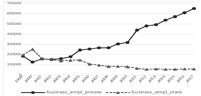
(11)GeoStat Business Statistics provide the number of persons employed by types of enterprise ownership[10] (state, private) from 1999-2017. These estimates are based on a statistical survey of enterprises.
Number of persons employed in the business sector by types of ownership, 1999-2017
Figure 8
Model results
Figure 9
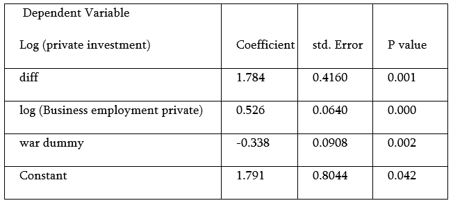
The coefficient on business employment is interpreted as follows: a one percent increase in employment brings about a 0.5 percent increase in private investment. This coefficient is of the expected sign (positive), and its magnitude is consistent with what has earlier been found in the empirical literature on the accelerator model (Alexiou (2009), Shapiro, Blanchard, and Lovell (1986)). Other coefficients in the model presented here also have the expected signs; in particular, the coefficient on the “marginal q” variable, showing that a 0.01 (1 percentage point) increase in the difference between real return and cost of capital would increase private investment by about 1.8%. As expected, the war effect had a negative 34% effect on private investment.
Conclusion
In this paper, we construct capital stock series for Georgia from 1996-2017 using the Perpetual Inventory Model. This paper describes the procedure and all the underlying assumptions in detail and publishes private and public capital stock time series data which is essential for economic growth models and productivity analysis, and in many other macroeconomic applications as demonstrated in the last two chapters of the paper. We found that the long-run growth rate of private investments is around 6.4% and it is 14.4% for public investment.
Using capital stock series, we estimated the return on capital for Georgia from 1996-2017. Results show that return on capital exhibits a large range of variation, between 7-26%. It increased from about 6% in 1996 to almost 26% in 2008, however it dropped significantly over the next two years as a result of the 2008 war with Russia and stabilized at around 14% over the last several years. The pattern for Georgia which is presented in our paper is consistent with findings in the literature for transitional economies.
In the last section of the paper, we use rate of return on capital series to try to understand what affected business investment demand in Georgia on a country level from 1999 to 2017. We find that private business employment, the difference between real return and cost of capital, and the war dummy are all significant determinants of private investment. A one percent increase in employment brings about a 0.5 percent increase in private investment, the increase in the difference between real return and cost of capital by 0.01 would increase private investment by about 1.8 percent, the war with Russia in 2008 shrank private investments by about 34% in 2008-2009 on average.
References:
- Alexiou C. (2009). Modelling Investment Behaviour: Emerging Evidence. The Indian Economic Journal 56(4): 21-36.
- Baldwin J., Gellatly G., Tanguay M., & Patry A. (2005, October). Estimating Depreciation Rates for the Productivity Accounts. In OECD Workshop on Productivity Measurement, Madrid Spain, October (pp. 17-19).
- Berlemann M., & Wesselhöft J. E. (2012). Estimating Aggregate Capital Stocks Using the Perpetual Inventory Method: New Empirical Evidence for 103 Countries (No. 125). Diskussionspapier, Helmut-Schmidt-Universität, Fächergruppe Volkswirtschaftslehre.
- Berlemann M., & Wesselhöft J. E. (2014). Estimating Aggregate Capital Stocks Using the Perpetual Inventory Method. Review of Economics, 65(1), 1-34.
- Burda M. C., Wyplosz C. (2017). Macroeconomics: A European Text. Oxford: Oxford University Press.
- Canale E., Lau A., Lee H., Manenti G., Owada K. (2017). Estimating the Rate of Return to Capital in the EU. LSE MPA Capstone Project.
- Chou N-T., Izyumov A., Vahaly J. (2015). Rates of Return on Capital Across the World: are they Converging? Cambridge Journal of Economics 40, no. 4 (2015): 1149-1166.
- Chou N-T., Izyumov A., Vahaly J. (2018). Capital Profitability and Economic Growth. Journal of Economics and Development Studies 6, no. 4 (2018): 12-18.
- Clark J. M. (1917). Business Acceleration and the law of Demand: A Technical Factor in Economic Cycles. Journal of Political Economy, 25(3), 217-235.
- De la Fuente A., & Domenech R. (2000). Human Capital and Growth: How Much Difference does Data Quality Make?. Economics Department Working papers no (262).
- Eurostat, European Commission, European system of accounts, ESA, 2010.
- Hall R. E., & Jorgenson D. W. (1967). Tax Policy and Investment Behavior. American economic review, 57(3), 391-414.
- Harberger A. C. (1978): Perspectives on Capital and Technology in Less Developed Countries. In: M. J. Artis and A. R. Nobay (Eds.): Contemporary Economic Analysis, London, 42–72.
- Harrod R.F. (1936). The Trade Cycle. Oxford: Oxford University Press.
- Harrod R.F. (1939). “An Essay in Dynamic Theory”, Economic Journal 49: 14-33.
- Hayashi F. (1982). Tobin's Marginal q and Average q: A Neoclassical Interpretation. Econometrica: Journal of the Econometric Society, 213-224.
- Hulten C. R., McCallum J. (Eds.). (1981). Depreciation, Inflation, and the Taxation of Income from Capital. Urban Institute Press.
- Levy D. (1995). Capital Stock Depreciation, Tax Rules, and Composition of Aggregate Investment. Journal of Economic and Social Measurement, 21(1), 45-65.
- Nehru V., Dhareshwar A. (1993). A New Database on Physical Capital Stock: Sources, Methodology, and Results. Revista de Análisis Económico–Economic Analysis Review, 8(1), 37-59.
- OECD Statistics (2001), Measuring Capital. OECD Manual. Measurement of Capital Stocks, Consumption of fixed Capital and Capital Services.
- Romer D. (2018). Advanced Macroeconomics.
- Shapiro M. D., Blanchard O. J., Lovell M. C. (1986). Investment, Output, and the Cost of Capital. Brookings Papers on Economic Activity, 1986(1), 111-164.
- Tvalodze S., Mkhatrishvili S., Mdivnishvili T., Tutberidze D., Zedginidze Z. (2016). The National Bank of Georgia’s Forecasting and Policy Analysis System. Macroeconomics and Statistics Department, Macroeconomic Research Division.
------------------------------------------------------------
[1] We are using the Perpetual Inventory Method assuming geometric depreciation at a constant rate, and at the same time we differentiate between different types of assets when constructing the depreciation rate parameter.
[2] https://matsne.gov.ge/ka/document/view/1648098?publication=0
[3] Statistics Canada – Catalogue no. 15-206 XIE, no. 005
[4] https://www.nbg.gov.ge/uploads/publications/fpas/FPAS%20Documentation.pdf
[5] https://www.geostat.ge/en/modules/categories/23/gross-domestic-product-gdp
[6] For illustrative purposes, in this study we simply use the Net Operating Surplus (NOS) to proxy for profits generated by capital. Different studies use slightly different approaches. For example, Chou, Izyumov and Vahaly (2015) also try to estimate capital profits by adding specific shares of the gross operating mixed income, which is the income of unincorporated enterprises owned by households (informal sector), to NOS. This approach assumes that in the informal sector output is divided between capital and labor incomes in the same proportion as in the corporate sector. This assumption, however, as the authors point out themselves, is somewhat arbitrary.
[7] For calculations, annual data from the Ministry of Finance on actually collected tax revenues are used (GeoStat)
[8] Consumption of fixed capital is defined as the decline during the accounting period in the current value of fixed assets used in the process of production as a result of physical depreciation, obsolescence, or accidental damages.
[9] Gross fixed capital formation of the private sector, including inventory investments, and excluding investment in dwellings. This variable is described in the Data section earlier in the paper.
[10] https://www.geostat.ge/en/modules/categories/326/statistical-survey-of-enterprises