Journal number 4 ∘ Nutsa Tokhadze ∘
Machine Learning and Econometric Approaches to FDI: FDI impact on Economic Growth in Georgia (1989-2023)

doi.org/10.52340/eab.2024.16.04.07

The primary objective of this paper is to analyze the impact of Foreign Direct Investment (FDI) on GDP in Georgia by applying both econometric (VECM) and machine learning (Random Forest) techniques. The paper compares the results from these two approaches, draws reliable conclusions, and offers recommendations for the government. To the best of our knowledge, no existing studies have utilized the Random Forest algorithm to analyze the effect of FDI on GDP in Georgia, and this paper addresses that gap.
The results from the VECM analysis show that FDI has a positive and statistically significant impact on GDP both in the short and long run. Similarly, the Random Forest model yields the same conclusion, with FDI demonstrating a positive effect, following the influence of gross capital formation. Based on these findings, the study offers recommendations to the Georgian government on strategies to attract more FDI and promote rapid economic growth.

Keywords: Foreign Direct Investments, Gross Domestic Product, Machine Learning, Random Forest, mice, Econometric.

Introduction

Data science, including artificial intelligence (AI), is advancing rapidly and becoming integral to numerous fields such as medicine, art, economics, and business. Almost every sector now relies on data, and utilizing it effectively has the potential to solve many problems across various domains. However, there is limited research that applies data science—particularly machine learning techniques—in economics and business, especially within the context of Georgia. This paper aims to fill that gap by applying machine learning methods to economic analysis, producing more reliable results, and offering valuable recommendations to the government. Notably, there are no existing studies that use the Random Forest machine learning approach to analyze the impact of foreign direct investment (FDI) on GDP in Georgia. Therefore, another key motivation of this study is to provide a foundation for future research and to encourage others to explore the use of machine learning techniques to investigate various economic topics related to Georgia.
One of the key effects of globalization is the movement of capital across borders. Foreign Direct Investment (FDI), defined as an investment where a foreign investor acquires at least 10% ownership in a company in another country, has become one of the most sought-after investment forms for many countries. FDI is especially crucial for developing countries, as it brings in foreign capital, technology, and expertise are considered essential drivers of rapid economic growth. As a result, policymakers often prioritize the development of favorable investment policies to attract FDI into their economies.
In Georgia, FDI has long been a central concern for policymakers, economists, and business leaders. There has been ongoing debate about strategies to boost FDI inflows into the country. Graph 1 below illustrates the net FDI inflows to Georgia from 1997 to 2023.

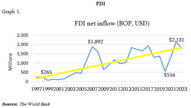
The yellow line on the graph represents trend. Figures indicate that the highest levels of FDI in Georgia occurred in 2007-1.8 Bill and 2022-2.1 Bill. A significant decline was observed in 2009, largely due to the Russia-Georgia war, and again in 2020 because of the COVID-19 pandemic. While net FDI fluctuated over the years, it showed a general upward trend. It is worthwhile to analyze FDI by country and economic sectors. Graph 2 displays the FDI from the top 10 investing countries in Georgia in 2023.

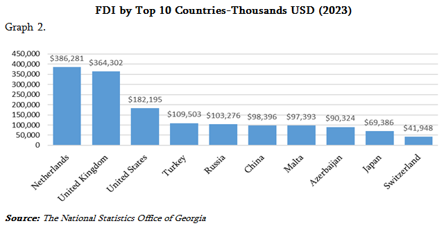
Based on the graph, the largest investors in 2023 were Netherlands with $386 million, followed by the UK ($364 million), the US ($182 million), Turkey ($109 million), and Russia ($103 million). It is also worth examining which sectors attracted the most investment. Chart 1 illustrates FDI by economic sectors in 2023.  

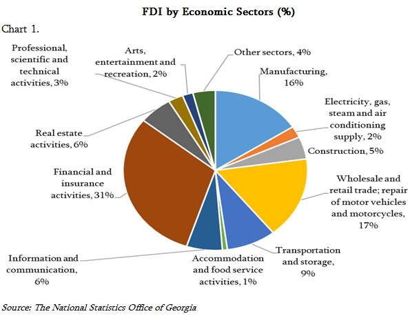
The largest share of FDI is directed towards financial and insurance activities (31%), followed by wholesale and retail trade (17%), manufacturing (16%), transportation and storage (9%), information and communication (6%), and real estate activities (6%).
While the positive impact of FDI on economic growth may seem evident, there is still considerable debate and ongoing research on the topic. Therefore, reviewing the literature on this subject is essential before proceeding with the modeling.

Literature Review

There are numerous studies examining the impact of Foreign Direct Investment (FDI) on economic growth in Georgia, but only a few have applied statistical analysis. Few studies have employed econometric techniques, and nearly none have applied machine learning approaches. However, econometric methods have been widely used in research on FDI and economic growth for other countries.
For example, a study conducted for Bangladesh applied an econometric model, specifically the Vector Error Correction Model (VECM), to investigate the impact of FDI, remittances, and foreign aid on economic growth from 1976 to 2021. The study concluded that all exogenous variables, including FDI, remittances, and aid, had a positive long-term impact on economic growth, although their short-term effects were not significant (Ummya et al., 2023).
A 2022 study analyzed the effects of public and private investments on economic growth in 39 developing countries from 1990 to 2019. Using panel data analysis, the study found that domestic private investment had a positive impact, while FDI showed a slightly negative effect on economic growth. It also identified that gross capital formation had a positive effect, whereas government expenditure had a negative impact on growth (Faruque, 2022,8).
Goken (2021, 95) examined the relationship between real economic growth and net FDI inflows in Turkey using VECM, covering the period from 1970 to 2019. The study found a positive but insignificant short-term impact of FDI on GDP and a significant but small effect of GDP on FDI. In the long run, the study revealed that while FDI did not significantly impact GDP, GDP had a positive impact on FDI in the long run.
სიხარულიძე, ჭარაია (2018) explored the theory of FDI and its experience in Georgia. They found that while FDI had a positive impact on economic growth, its long-term effect was not stable. The study noted that foreign companies were not well integrated with local firms, and the lack of competitiveness, qualifications, and strong linkages between the two hindered more sustainable benefits from FDI. To maximize the impact of FDI, the study recommended appropriate investment policies for Georgia.
Hlavacek et al. (2016, 294-303) examined the relationship between FDI and economic growth in Central and Eastern Europe (CEE) from 2000 to 2012. Their panel data model showed a significant positive impact of FDI on economic growth, which was particularly pronounced as these countries joined the European Union, accelerating their integration and attracting more FDI.
Simionescu (2016, 187-213,) conducted a study for 28 European Union countries, focusing on the impact of FDI on GDP growth from 2008 to 2014. Using a panel data approach with Bayesian methods, the study concluded that overall, FDI had a positive effect on economic growth in the EU. However, for some countries, FDI did not contribute significantly to growth. For those countries, the study suggested the implementation of targeted economic policies, such as tax reductions and better legislative environments.
Pharjiani (2015, 3988-3996) investigated the sectoral impact of FDI on economic growth in 10 CEE countries from 1995 to 2012. The study used various econometric methods, including Ordinary Least Squares (OLS), Random Effects (RE), and Fixed Effects (FE), and found a positive link between FDI and economic growth in each sector, with FDI contributing to increased productivity.
Albulescu (2014, 507-512) researched the impact of both inward and outward FDI and Foreign Portfolio Investment (FPI) on economic growth in CEE countries using a panel Generalized Method of Moments (GMM) approach. The study, which covered 2005 to 2012, found that both inward and outward FDI, as well as FPI, positively affected economic growth.
Acaravaci et al. (2012, 52-67) explored the long-run causal relationships between FDI, exports, and economic growth in 10 transition European countries, including Bulgaria, Czech Republic, Estonia, and others. Using VECM and Granger causality tests, the study concluded that there were both short- and long-term causal relationships between FDI, exports, and economic growth in four of these countries.
Batten et al. (2009,1621-1641) studied the relationship between FDI and economic growth in 79 countries from 1980 to 2003. The study found that FDI had a positive impact on economic growth in countries with higher education levels, developed stock markets, and openness to international trade.
Stanisic (2008) examined FDI's impact on economic growth in seven Southeastern European countries from 1997 to 2005. The study found no positive correlation between FDI and economic growth, attributing this to the transition period these countries were undergoing, which hindered increases in production and employment which abate the positive impact of FDI.
Another study by Moudatsou (2003, 689-707) analyzed FDI’s impact on economic growth in the EU from 1980 to 1996. The research concluded that while the impact of FDI on growth differed across countries, there was a positive overall effect when the data was pooled together.

Data and Methodology

Exploratory & Initial Data Analysis / Overview of the Data
The data used in the modeling was collected from the World Bank covering a period of 35 years, from 1989 to 2023. Variables such as the Consumer Price Index (CPI), employment-to-population ratio, labor force participation rate, etc. were also considered, but the final selection of variables were based on their importance and correlations, also avoiding high multicollinearity. The final dataset includes the key economic variables such as:
• GDP - GDP per capita (USD)
• FDI – FDI, net inflows per capita (USD)
• GCF - Gross Capital Formation per capita (USD)
• GOVEX - General Government Final Consumption Expenditure (% of GDP)
• TRBAL - Trade Balance on goods and services (% to GDP)
• POPGR - Population Growth Rate (annual %)
The dataset contained some missing values, and an imputation method was applied to address this issue. Missing data analysis involves various approaches, with the choice of method depending on the patterns and mechanisms of the missingness. The pattern of missing data indicates where the missing values occur within the dataset, while the mechanism provides insight into the reasons behind the data's absence.
There are three primary mechanisms for missing data: Missing Completely at Random (MCAR), Missing at Random (MAR), and Missing Not at Random (MNAR). The nature of the missing data mechanism influences the selection of appropriate analysis methods. (Little et.al 2019).
Common imputation techniques include: Unconditional mean imputation, where missing values are replaced by the overall mean of the observed values; Conditional mean imputation, or Regression imputation, where missing values are predicted from other variables using regression models; Stochastic regression imputation, which refines regression imputation by adding random noise to predicted values; Hot deck imputation, where missing values are filled using values from similar individuals in the dataset; Cold deck imputation, which uses previously collected data to fill in missing values; Last Observation Carried Forward (LOCF) imputation, often used in longitudinal studies, where the last observed value is carried forward to fill in missing data. (Little et al. 2019).
The R statistical software provides various packages for multiple imputation, each using different algorithms. One widely used package is mice (Multiple Imputation by Chained Equations), which generates multiple completed datasets by imputing missing values according to a specified method, applies the substantive statistical model to each dataset, and combines the results using Rubin’s rules. (Van Buuren, et al. 2011, 1-67).
Within the mice framework, Random Forest (RF) is one of the available imputation methods. Random Forest Multiple Imputation is particularly effective for time series data under certain conditions. It excels at capturing non-linear and complex relationships between variables, managing high-dimensional datasets without overfitting, and adapting to trends or seasonality in the data. When the data is MAR or MCAR, Random Forest can produce robust estimates, especially when variable interactions are present or the dataset is large. (Gqmez-Méndez et.al, 2023, 1924-1949).
In this study, the relationship between the independent and dependent variables is non-linear and complex, with the missing data mechanism being MAR and variables interacting with one another. Therefore, the Random Forest method within the mice package was applied for imputing missing data, and the final time series dataset is presented in Graph 3.

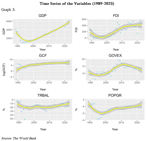
The blue points on the graphs represent the data points, while the yellow line indicates the trend. Over the past 35 years, several key political and economic events have shaped Georgia, including 1991, when the Soviet Union collapsed; 2003, when the Rose Revolution led to the rise of the 'National Movement'; 2008, when the Russian-Georgian war occurred; and 2012, when the 'Georgian Dream' party took office following a change in government.
GDP and FDI per capita have the same trend After 1994, they both increased. The Gross Capital Formation per capita (GCF), followed the path of GDP per capita, and the log was taken to stabilize the variance, reduce multicollinearity, and make it easier for modeling. Government Expenditure (GOVEX), as a percentage of GDP, showed an upward trend from 1995 to 2011 but decreased after 2012. The trade balance (TRBAL), as a percentage of GDP, was negative and increased (in absolute values) until 1995, after which it showed a slight positive trend, reflecting a decrease in absolute values on average. The annual population growth rate (POPGR) dramatically declined between 1993 and 1995 due to the collapse of the Soviet Union, then began to rise, and remained relatively stable from 2012 onward.

Methodology

Unite Root test –Augmented Dicky Fuller and PPC test
The time series stationarity is crucial for econometric modeling. A time series is stationary if its mean and variance don’t change across time. Non-stationary time series can lead to misleading correlations, suggesting relationships between variables that do not actually exist, which can result in incorrect conclusions about causation. Moreover, non-stationary data can cause parameters to change over time, making it difficult to interpret the model's results and potentially diminish the predictive accuracy.
There are two primary approaches for testing stationarity: parametric and non-parametric methods (Masliah). This paper emphasizes a unit root test, which is a parametric approach. The unit root test detects the unit root in a time series. If the solution to the characteristic equation is equal to (1), then the time series exhibits a unit root, indicating that the data is non-stationary; conversely, if it is not (1), the data is stationary. (Afriyie, et al. 2020, 656-664).
Common unit root tests include the Dickey-Fuller test (DF) which tests the null hypothesis that a unit root is present in the series; the Augmented Dickey-Fuller (ADF) test, which extends the DF test by including lagged terms to account for autocorrelation (Mushtaq, 2011); and the Phillips-Perron (PP) test, which is similar to the ADF but adjusts for autocorrelation and heteroscedasticity in the errors. (Leybourne, et al. 1999, 51-61). This paper focuses on the ADF and PP tests to assess the stationarity of the data.

Cointegration Test

While each individual time series may not be stationary, they can be cointegrated meaning their linear combination could be stationary, indicating that the series move together and exhibit long-term dependence. If the time series data is found to be cointegrated, it suggests that the series can be modeled together and used for forecasting. In such cases, models such as Error Correction Models (ECM) or Vector Error Correction Models (VECM) can be built. Cointegration methods are particularly useful in fields like financial markets, macroeconomic modeling, and econometric time series analysis, for example, when examining the long-term relationships between variables such as GDP, unemployment, and inflation. (Ssekuma, 2011)
There are three main types of cointegration tests: Engle-Granger Two-Step Method: This method estimates the relationship between the two time series data using Ordinary Least Squares (OLS) regression and then tests the residuals of the regression for stationarity, typically using the Augmented Dickey-Fuller (ADF) test. If the residuals are stationary, the series are considered cointegrated. A second method Johansen Cointegration Test uses a more general approach than the Engle-Granger method and uses maximum likelihood estimation to identify the cointegration among multiple time series data. The third method is the Phillips-Ouliaris Cointegration Test; this method is similar to the Engle-Granger test but uses a slightly different approach for calculating the test statistics. (Ssekuma, 2011).
Since this study involves multiple variables, the Johansen Cointegration Test was performed to assess the cointegration before applying the Vector Error Correction Model (VECM).

Vector Error Correction Model (VECM)

Vector Error Correction Models (VECM) are used to model cointegrated, non-stationary time series data. They are extensions of Vector Autoregressive (VAR) models and are designed to capture both short-term dynamics and long-term equilibrium, making them more robust than standard VAR models. VECM is particularly useful for handling multiple variables with complex interrelationships, making them ideal for multivariate analysis.
VECM accounts for deviations from long-term equilibrium and corrects these over time. According to the model, lagged changes in the variables, along with the error correction term, explain short-term fluctuations in the dependent variables. The error correction term restores the long-term relationship and indicates how quickly variables return to equilibrium after a shock. Additionally, VECM models include lagged differences of the time series, ensuring that temporary shocks and changes are incorporated into the system. (Lxtkepohl, 2005, 237-267).
The general mathematical formulation of the VECM can be expressed as:

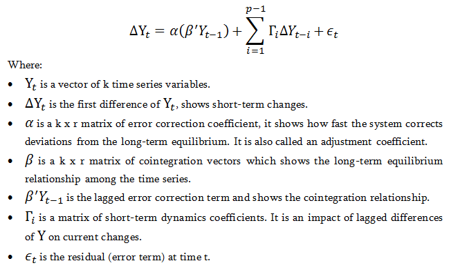
To implement a VECM, the first step is to test whether the time series data are cointegrated, typically using the Johansen Cointegration Test. Only cointegrated variables should be included in the VECM. Next, the appropriate number of lags should be selected using model selection criteria such as AIC (Akaike Information Criterion), HQ (Hannan-Quinn Information Criterion), SC (Schwarz Criterion or BIC - Bayesian Information Criterion) and/or FPE (Final Prediction Error). Finally, the VECM is estimated by incorporating both long-term and short-term equilibrium relationships, along with estimating the coefficients for short-term changes and the error correction term. (Lxtkepohl, 2005, 237-267).
In conclusion, the VECM is a useful econometric tool for modeling and forecasting cointegrated time series data and it is particularly valuable in financial and economic modeling, where long-term relationships are anticipated. Therefore, this model has been applied in this paper.

Random Forest

Random Forest is a machine learning algorithm typically used for classification and regression tasks. It works by constructing multiple decision trees, aggregating their results, and making final predictions. Each tree is trained on a random subset of the data, and at each split, a random subset of features is considered. This randomness helps to minimize overfitting and enhance the model’s ability to generalize. When applied to time series data, Random Forest functions like other supervised learning methods, but it requires special attention to the temporal structure of the data to prevent future information from being inadvertently incorporated into the model and to prevent data leakage. (Tyralis, et al. 2017)
Before modeling, features need to be created, such as lagged values of existing variables. Additionally, rolling windows can be used to capture short-term trends or seasonal patterns. If the time series exhibits strong seasonal or trend components, features like months, days, or weeks can be added. For detrending and removing long-term dependencies, differencing the data is another effective approach. Once the features are created, the model can be trained on the training data and evaluated on the test data. Common evaluation metrics for time series models include Mean Absolute Error (MAE), Root Mean Squared Error (RMSE), Mean Absolute Percentage Error (MAPE), and R-squared. (Tyralis, et al. 2017).
Unlike traditional time series models such as ARIMA, Random Forest does not assume a linear relationship between past and future values. It can also handle missing data without the need for imputation and does not require the data to be stationary. This makes Random Forest a powerful tool for modeling time series data, as it can detect complex, non-linear relationships between multiple variables and provide accurate forecasts. Since the variables in this article exhibit non-linear relationships Random Forest model was applied to detect short, long-run, and nonlinear relationships among the variables.

Results

Econometric Results: Cointegration Test and VECM
Before modeling, it is important to check the stationarity of the time series data. The Augmented Dickey-Fuller (ADF) and Phillips-Perron (PP) tests were used for this purpose, specifically the adf.test and pp.test functions in R.
If the absolute value of the t-statistic exceeds the critical value, the null hypothesis (which states that the data is non-stationary) can be rejected. In other words, if the p-value is smaller than the significance level, the null hypothesis of non-stationarity is rejected. The tests were conducted at a 5% significance level. The results of the ADF test indicated that TRBAL and POPGR were stationary at the level, while the other variables were not. However, all variables became stationary after taking the first difference. In contrast, the PP test revealed that none of the variables were stationary at the level, but all were stationary after the first difference. The results from the PP test were considered more reliable, as the p-values for almost all variables at the first difference were below 0.01, confirming they were stationary at the first difference (I(1)). Therefore, the PP test results were used as the primary reference.
Given that the time series data was non-stationary at the level but stationary at the first difference (I(1)), a Johansen Cointegration Test and VECM analysis was performed.
The study examines multiple variables, thus before conducting VECM, the Johansen Cointegration Test was performed, and the test statistics and critical values are presented in Table 2.

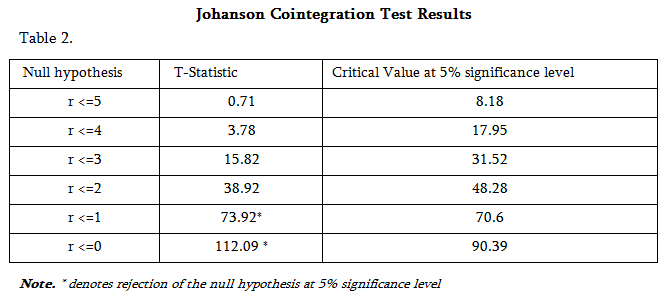
The results indicate that for r≤0r the t-statistic is 112.09, which exceeds the critical value of 90.39. Therefore, the null hypothesis (Ho) that no cointegration vector exists is rejected. For r≤1, the t-statistic of 73.92 is greater than the critical value of 70.6, leading to the rejection of the null hypothesis that at most one cointegration vector exists. However, for r≤2, the test statistic of 38.92 is less than the critical value of 48.28, meaning the null hypothesis (Ho) that at most two cointegration vectors exist fail to be rejected.
Thus, the results suggest that there are at most two cointegrating vectors, indicating a long-run relationship among the variables. Implementing a Vector Error Correction Model (VECM) would provide a more detailed explanation of these results.
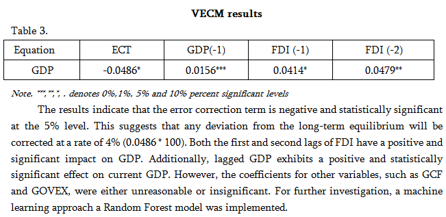
The appropriate number of lags 2 were selected using model selection criteria such as AIC, HQ, SC, and FPE and only cointegrated variables were included in the VECM. The results of VECM are shown in table 3, which shows only the significant variables in the model.

Machin Learning Results
The Random Forest models were trained to predict GDP using FDI, government expenditure, gross capital formation, and other economic variables. All variables were tested in the model, and after considering model accuracy, as well as the risks of underfitting and overfitting, the most relevant variables were selected. Two models were trained: one without lags and one with lags.

Random Forest without Lags
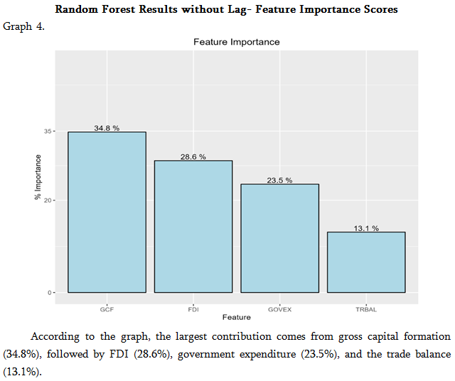
This model does not include lags. To prevent overfitting, a maximum of four variables were selected, and GDP was regressed on FDI, GOVEX, GCF, and TRBAL. The model demonstrated a strong performance, with an R-squared of 88% and an RMSE of 0.25. The feature importance results are shown in Graph 4.

Random Forest with Lags

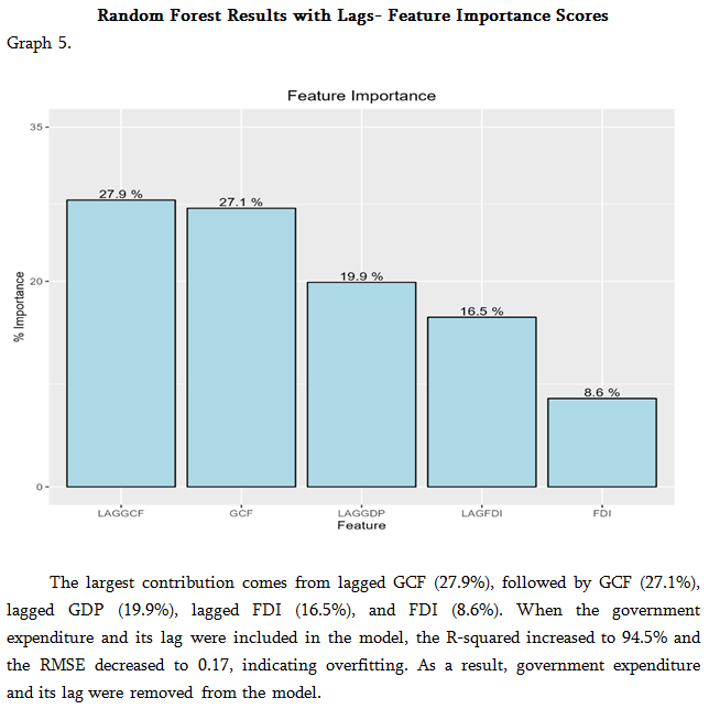
In the second model, lags were added to the data, and the trade balance (TRBAL) and government expenditure (GOVEX) variables were removed to avoid overfitting. GDP was regressed on FDI, GCF, and their lags, as well as the lag of GDP itself. The model showed a strong performance, with an R-squared of 90% (slightly overfitting) and an RMSE of 0.22. The feature importance results are shown in Graph 5.

Conclusions and Discussions

The study examined the impact of Foreign Direct Investment (FDI) per capita on GDP per capita in Georgia over a 35-year period from 1989 to 2023. Both econometric and machine learning approaches were employed, incorporating key economic variables such as Gross Capital Formation per capita (GCF), Government Expenditure as a percentage of GDP (GOVEX), Trade Balance as a percentage of GDP (TRBAL), and Population Growth Rate (POPGR) alongside FDI per capita. Although other variables were also considered, only the most relevant ones were included in the final model.
For the econometric analysis, the data was first tested for stationarity, followed by a cointegration test. A Vector Error Correction Model (VECM) was then developed. The results from the VECM indicated that the first lag of GDP per capita has a positive and statistically significant effect on current GDP per capita, and both the first and second lags of FDI per capita have a positive and significant impact on GDP per capita. This suggests that FDI per capita positively influences per capita economic growth in the long term. However, the coefficients for other variables, such as GCF, GOVEX, POPGR, and TRBAL, were found to be insignificant, implying that the VECM may not have captured any non-linear relationships.
To further explore these findings, a machine learning approach was applied, specifically using the Random Forest model, both with and without lags. The models exhibited some overfitting, leading to the removal of less important variables. Both versions of the model performed well, with an R-squared above 80% and a Root Mean Square Error (RMSE) between 0.17 and 0.22. The Random Forest model without lags indicated that the largest impact on GDP per capita comes from GCF per capita (34.8%), followed by per capita net FDI (28.6%), government expenditure (% of GDP)- 23.5%, and the trade balance (% of GDP) -13.1%. This suggests that FDI has a significant positive impact on economic growth, but its effect is secondary to that of gross capital formation.
In the lagged model, government expenditure and trade balance were removed due to overfitting concerns. The remaining variables—GCF, FDI, and their lags—were included, along with the lag of GDP. The results showed that lagged gross capital formation (GCF) had the largest impact on GDP per capita (27.9%), followed by current GCF (27.1%), lagged GDP (19.9%), lagged FDI (16.5%), and current FDI (8.6%). As lots of other studies, the results of this paper also indicate that FDI has both a short-term and long-term positive effect on GDP per capita.
Based on these findings, the government should prioritize creating an investor-friendly environment to attract more foreign direct investment (FDI). The main barriers to FDI in Georgia include:
• Underdeveloped capital and bond markets
• High interest rates on financial resources
• Political and economic instability
• A small market size that is unattractive to large companies
• A low level of education and a less qualified workforce
• Concerns over the fairness and objectivity of the judicial system and insufficient protection of property rights
• Poor infrastructure, particularly in rural areas
To address these issues and encourage greater FDI inflow, the government should focus on improving these factors, which will ultimately stimulate economic growth in Georgia.
Comparing econometric (VECM) and Machine learning (Random Forest) approaches, the latest seems give more robust and complete results for this analysis, but given the complexity of econometric and machine learning techniques, there is potential for further research using nonlinear econometric models, such as Threshold Autoregressive Models (TAR), Smooth Transition Autoregressive Models (STAR), Nonlinear Cointegration Models, Nonlinear Error Correction Models (NECM) and Granger Causality Test. In the realm of machine learning, future studies could explore advanced techniques like Gradient Boosting Machines (GBM), including XGBoost (an optimized and efficient version of GBM), LightGBM (a faster variant using histogram-based approaches), CatBoost (which handles categorical variables effectively), and Long Short-Term Memory (LSTM) networks. Other econometric and machine learning models, when used together, could provide more valuable insights to further enhance the analysis. Typically, the most accurate results are obtained by applying both approaches, rather than relying on just one.

ლიტერატურა:
References:
• სიხარულიძე დ. ჭარაია ვ. (2018). „პირდაპირი უხოური ინვესტიციები: თეორია და საქართველოს გამოცდილება“. გამომცემლობა „უნივერსალი“.
• Sikharulidze D. Charaya V. (2018). „pirdapiri utskhouri investitsiebi: sakartvelos teoria da gamotsdileba“. [“Foreign Direct Investments. Theory and Georgian Experience”. Publishing House “Universal”.] in Georgian
• Acaravci A., & Ozturk I. (2012). Foreign Direct Investment, Export and Economic Growth: Empirical Evidence from New EU Countries. Romanian Journal of Economic Forecasting, 2(2), 52-67.
• Afriyie J. K., Twumasi-Ankrah S., Gyamfi K. B., Arthur D. & Pels W. A. (2020). Evaluating the Performance of Unit Root Tests in Single Time Series Processes. Mathematics and Statistics, 8(6), 656-664.
• Ahamed F. (2022). Impact of Public and Private Investments on Economic Growth of Developing Countries (Master's thesis, Northern Illinois University).
• Albulescu C. T. (2015). Do Foreign Direct and Portfolio Investments Affect Long-term Economic Growth in Central and Eastern Europe?. Procedia Economics and Finance, 23, 507-512.
• Batten J. A., & Vo X. V. (2009). An Analysis of the Relationship between Foreign Direct Investment and Economic Growth. Applied Economics, 41(13), 1621-1641.
• Gokmen O. (2021). The Relationship between Foreign Direct Investment and Economic Growth: A case of Turkey. arXiv preprint arXiv:2106.08144.
• Gómez-Méndez I. & Joly E. (2023). Regression with Missing Data, a Comparison Study of Techniques based on Random Forests. Journal of Statistical Computation and Simulation, 93 (12), 1924-1949.
• Hlavacek,P. & Bal-Domanska B. (2016). Impact of Foreign Direct Investment and Economic Growth in Central and Eastern European Countries. Engineering Economics, 27(3), 294-303.
• Leybourne S. & Newbold P. (1999). On the Size Properties of Phillips–Perron Tests. Journal of Time Series Analysis, 20(1), 51-61.
• Little R. J. & Rubin D. B. (2019). Statistical Analysis with Missing Data (Vol. 793). John Wiley & Sons.
• Lütkepohl H. (2005). "Vector Error Correction Models." New Introduction to Multiple Time Series Analysis, 237-267.
• Moudatsou, A. (2003). Foreign Direct Investment and Economic Growth in the European Union. Journal of Economic Integration, 689-707.
• Mushtaq R. (2011). Augmented Dickey Fuller test.
• Pharjiani S. (2015). "Foreign Direct Investment on Economic Growth by Industries in Central and Eastern European Countries." Int. J. Econ. Manag. Eng 9 3988-3996.
• Salma U., Khan M. F. H. & Billah M. M. (2023). Foreign Capital and Economic Growth: Evidence from Bangladesh. arXiv preprint arXiv:2312.04695.
• Simionescu M. (2016). The Relation between Economic Growth and Foreign Direct Investment during the Economic Crisis in the European Union. Zbornik Radova Ekonomskog Fakulteta u Rijeci: časopis za ekonomsku teoriju i praksu, 34(1), 187-213.
• Ssekuma R. (2011)."A Study of Cointegration Models with Applications." University of South Africa.
• Stanisic N. (2008). Do Foreign Direct Investments Increase the Economic Growth of Southeastern European Transition Economies?. South-Eastern Europe Journal of Economics, 6(1).
• Tyralis H., & Papacharalampous G. (2017). Variable Selection in Time Series Forecasting Using Random Forests. Algorithms, 10(4), 114.
• Van Buuren S., & Groothuis-Oudshoorn, K. (2011). mice: Multivariate Imputation by Chained Equations in R. Journal of Statistical Software, 45, 1-67.

---